
This article discusses the reflections on a transmission line terminated with either an RL or an RC load. The detailed analytical derivations are verified through the HyperLynx simulations and laboratory measurements.
1.1 Reflections at the RL Load – Analysis
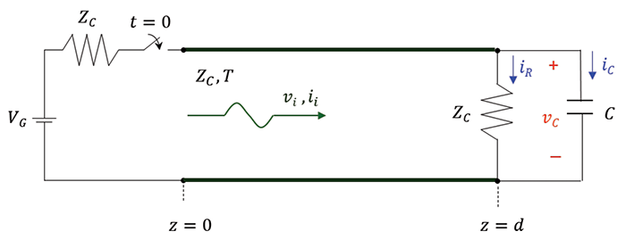
Consider the circuit shown in Figure 1.1, where the transmission line of length d is terminated by an RL load. (Reflections at the purely inductive load are discussed in [1]).
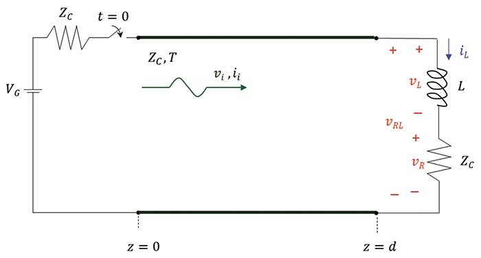
Note that the load resistor value is equal to the characteristic impedance of the transmission line; it is also assumed that the initial current through the inductor is zero, iL(0_) = 0.
When the switch closes at t = 0, a wave originates at z = 0, [2], with
![]() (1.1a)
(1.1a)
![]() (1.1b)
(1.1b)
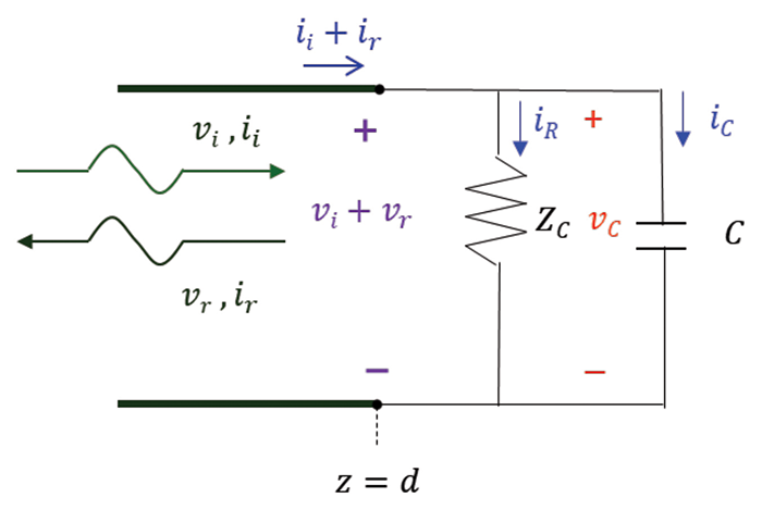
and travels towards the load. When this wave arrives at the load, (at the time t = T), the reflected waves, vr and ir are created. This is shown in Figure 1.2.
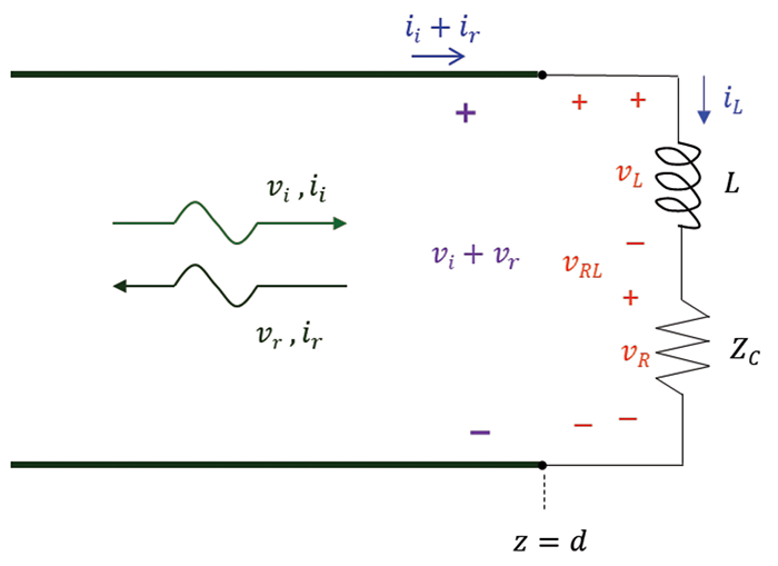
The reflected current wave is related to the reflected voltage wave by
![]() (1.1c)
(1.1c)
KVL and KCL at the load produce
![]() (1.2a)
(1.2a)
![]() (1.2b)
(1.2b)
Our initial goal is to determine the reflected voltage vr(t) at the location z = d, i.e., vr(d,t). The ultimate goal is to determine the total voltage at the load, vRL(d,t). From Eq. (1.2a) we obtain the inductor voltage as
![]() (1.3)
(1.3)
The load resistor voltage can be obtained from
![]() (1.4)
(1.4)
Using Eqns. (1.1a) and (1.4) in Eq. (1.3) produces
![]() (1.5)
(1.5)
The differential v-i relationship for the inductor is
![]() (1.6)
(1.6)
Utilizing Eqns. (1.2b) and (1.6) in Eq. (1.5) we get
![]() (1.7)
(1.7)
Using Eq. (1.1b) and (1.1c) in Eq. (1.7) we have
![]() (1.8)
(1.8)
Since VG and ZC are constant Eq. (1.8) reduces to
![]() (1.9)
(1.9)
This differential equation needs to be solved for vr(t), for t > T, subject to the initial condition vr(t = T). Let’s determine this initial condition. Using Eqns. (1.1a) and (1.1c) in (1.2b) gives
![]() (1.10)
(1.10)
Evaluating t = T it at , we get
![]() (1.11)
(1.11)
Since the current through the inductor cannot change instantaneously, we have iL(T), and thus
![]() (1.12)
(1.12)
Now we are ready to solve Eq. (1.9), subject to the initial condition in Eq. (1.12):
![]() (1.13)
(1.13)
First, let’s rewrite this equation in a standard form:
![]() (1.14)
(1.14)
or
![]() (1.15)
(1.15)
where
![]() (1.16)
(1.16)
The solution of Eq. (1.16) was derived in [3] as
![]() (1.17)
(1.17)
Utilizing Eqns. (1.12) and (1.16) in Eq. (1.17) we obtain
![]() (1.18)
(1.18)
The total voltage across the RL load is
![]() (1.19a)
(1.19a)
or
![]() (1.19b)
(1.19b)
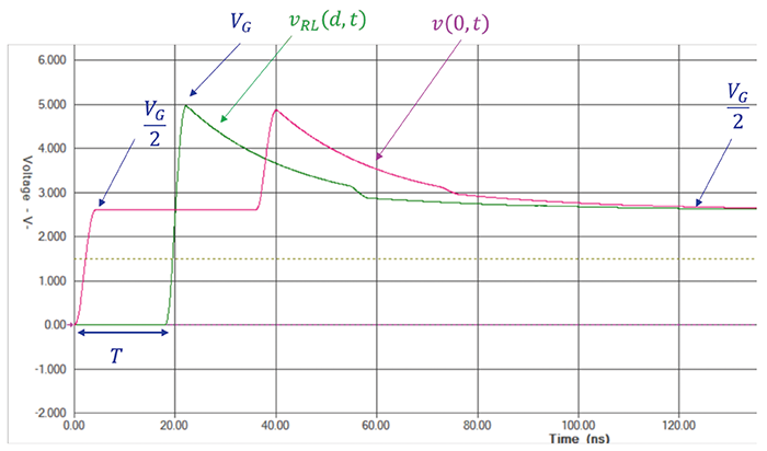
Equation (1.19b) predicts that at t = T, the voltage at the load rises from zero to VG, and then decays exponentially to VG/2. Let’s verify these observations through simulations and measurements.
1.2 Reflections at the RL Load – Simulation
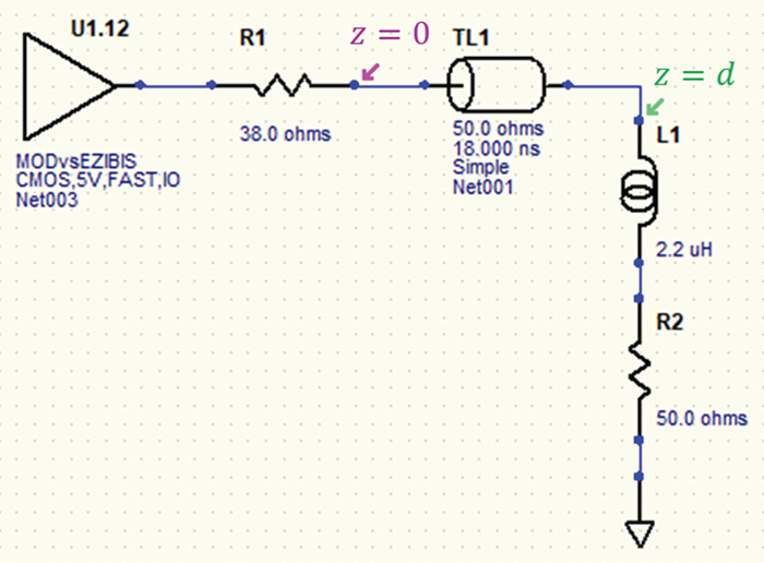
Figure 1.3 shows the HyperLynx schematic of the transmission line terminated in an RL load.
The simulation results are shown in Figure 1.4.
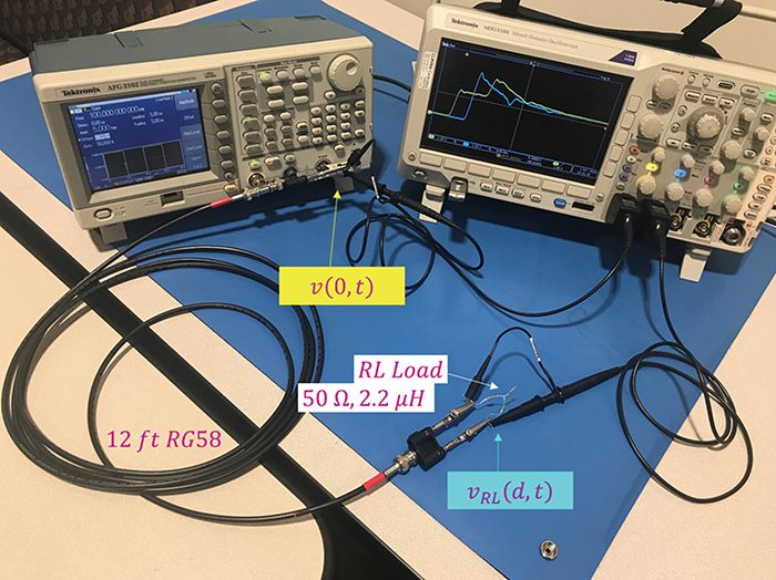
1.3 Reflections at the RL Load – Measurements
The measurement setup and the results are shown in Figure 1.5.
The measurement results are shown in Figure 1.6.
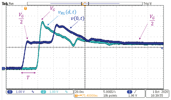
Note that the measurement results verify the simulation and the analytical results.
2.1 Reflections at the RC Load – Analysis
Consider the circuit shown in Figure 2.1 where the transmission line of length d is terminated by an RC load. (Reflections at the purely capacitive load are discussed in [1]).
Note that the load resistor value is equal to the characteristic impedance of the transmission line; it is also assumed that the initial voltage across the capacitor is zero, vC(0_) = 0.
When the switch closes at t = 0, a wave originates at z = 0, with the initial voltage and current values given by Eqns. (1.1a) and (1.1b); this wave travels towards the load. When the wave arrives at the load, (at the time t = T), the reflected waves, vr and ir are created. This is shown in Figure 2.2.
The reflected current wave is related to the reflected voltage wave by Eq. (1.1c). KVL and KCL at the load produce
![]() (2.1a)
(2.1a)
![]() (2.1b)
(2.1b)
Our initial goal is to determine the reflected voltage vr(t) at the location z = d, i.e., vr(d, t). The ultimate goal is to determine the voltage at the load, vC(d, t). From Eq. (2.1b) we obtain the capacitor current as
![]() (2.2)
(2.2)
The load resistor current can be obtained from
![]() (2.3)
(2.3)
Using Eqns. (1.1b), (1.1c) and (2.3) in Eq. (2.2) produces
![]() (2.4)
(2.4)
The differential v-i relationship for the capacitor is
![]() (2.5)
(2.5)
Utilizing Eqns. (1.1a) and (2.4) in Eq. (2.5) we get
![]() (2.6)
(2.6)
Since VG is constant Eq. (2.6) reduces to
![]() (2.7)
(2.7)
This differential equation needs to be solved for vr(t), for t > T, subject to the initial condition vr(t = T). Let’s determine this initial condition. Using Eq. (1.1a) in (2.1a) gives
![]() (2.8)
(2.8)
Evaluating it at t = T, we get
![]() (2.9)
(2.9)
Since the voltage across the capacitor cannot change instantaneously, we have vC(T) = 0, and thus
![]() (2.10)
(2.10)
Now we are ready to solve Eq. (2.7), subject to the initial condition in Eq. (2.10):
![]() (2.11)
(2.11)
First, let’s rewrite this equation in a standard form:
![]() (2.12)
(2.12)
This equation is in the form of Eq. (1.15), with
![]() (2.13)
(2.13)
The solution of Eq. (2.13) is of the form presented in Eq. (1.17). Utilizing Eqns. (2.10) and (2.13) in Eq. (1.17) we obtain
![]() (2.14)
(2.14)
The total voltage across the RC load is
![]() (2.15a)
(2.15a)
or
![]() (2.15b)
(2.15b)
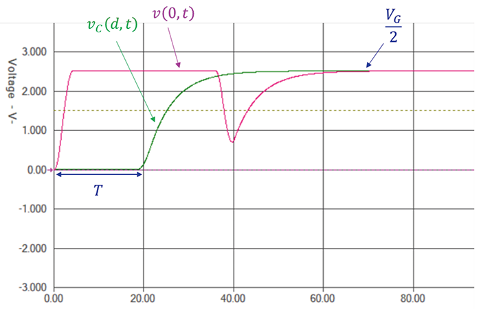
Equation (2.15b) predicts that at t = T, the voltage at the load is zero and increases exponentially to VG/2. Let’s verify these observations through simulations and measurements.
2.2 Reflections at the RC Load – Simulation
Figure 2.3 shows the HyperLynx schematic of the transmission line terminated in an RC load.
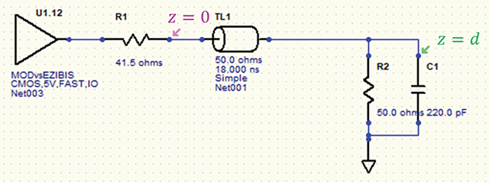
The simulation results are shown in Figure 2.4.
2.3 Reflections at the RC Load – Measurements
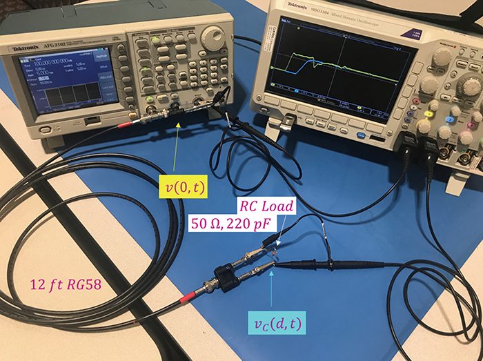
The measurement setup and the results are shown in Figure 2.5.
The measurement results are shown in Figure 2.6.
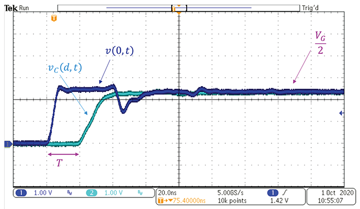
Note that the measurement results verify the simulation and the analytical results.
References
- Adamczyk, B., “Transmission Line Reflections at a Reactive Load,” In Compliance Magazine, December 2018.
- Adamczyk, B., “Transmission Line Reflections at a Resistive Load,” In Compliance Magazine, January 2017.
- Adamczyk, B. Foundations of Electromagnetic Compatibility with Practical Applications, Wiley, 2017.